Linear and Quadratic Approximation

CHAPTER 2 SECTION 9
August 1999

1. In this section

One of the most important applications of the derivative is the construction of lines (or polynomials
of some fixed degree) that approximate a complex function near some point (we call this
local approximation, and in the case of lines, linear approximation). In this section, we develop
formulas for the construction of both approximating lines and parabolas for functions.

2. The tangent line and linear approximation

The single most important thing to remember about the derivative is that it tells us how best to
(locally) approximate a function by a straight line (the tangent line to the graph). The slope of
this line is also referred to as the instantaneous rate of change of the function (at the point under
consideration).

We have already discussed the fact that the tangent line is the best local approximation to a
function. The equation of the tangent line to the graph of a function f at a point (x₀, f(x₀)) is:
y = f(x₀) + f'(x₀) (x - x₀) .

So, the idea is that, for x close to x₀,
f(x) ≈ f(x₀) + f'(x₀) (x - x₀) .

This is called linear approximation; we are approximating a function with a line.

Let’s remind ourselves how this works by looking at an example. Suppose we consider the
function
f(x) = sqrt(x).

Then

We know the exact value of both f and f' at any perfect square (1, 4, 9, 16, ...), and can readily
find the equation of the tangent line to the graph at any point corresponding to one of these.

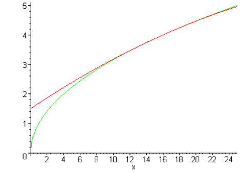
Let’s look at the tangent line at the point (16,4), together with the original function

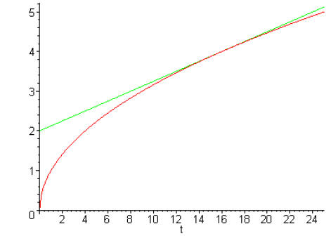
We see that the tangent line remains close to the graph of the function (is a good approximation)
close to the point (16,4). We can use the simpler equation of the tangent line to approximate the
function.

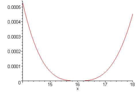
Here is a plot of the difference between the two:

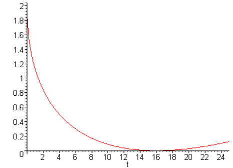
Note that the approximation appears to be very good between 14 and 18:

Note that, at the point (x₀, f(x₀)), the derivative of the function that defines the tangent line has
the same value as the derivative of f at that point. That’s really obvious since we construct the
tangent line with slope f' (x₀). The point is that the tangent line matches the original funcion and
its derivative at the point (x₀, f(x₀)).

3. Quadratic approximation

We can extend this notion of local approximation to higher orders. The next step is to consider
quadratic approximations.

For a function f, we wish to construct a quadratic polynomial which is the best approximation
to f near a given point (x₀, f(x₀)). Following the reasoning above, we want to find a quadratic
function which passes through (x₀, f(x₀)) and has the same first and second derivatives as f at
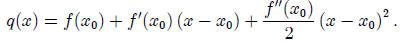
that point. This is best done by writing a quadratic in the form:
q(x) = c + b (x − x₀) + a (x − x₀)² .

Remember that we want q and f to satisfy
q (x₀) = f (x₀)
q'(x₀) = f'(x₀)
q"(x₀) = f" (x₀) .

The first condition immediately yields c = f(x₀).
Since
q'(x) = b + 2a(x - x₀),

the condition q'(x₀) = f'(x₀) requires that we choose
b = f'(x₀) .

Note that the linear piece of our quadratic function is the same as the tangent line. Finally, since
q"(x) = 2a, the condition q" (x₀) = f" (x₀) means that we must take

So, our quadratic approximation becomes

In our example above, we looked at the linear approximation to the graph of f(x) = √x at the
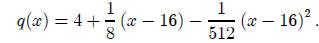
point (16,4). Since

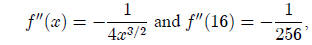
the quadratic approximation at the same point is

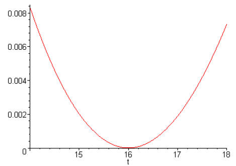
Let’s look at a plot of this, together with a plot of f, to see how close the approximation is.

This approximation looks very good near (16,4). Let’s look at the plot of the difference over a
smaller interval.

Comparing this approximation to the linear approximation, it appears that we have improved the

accuracy by about a factor of 10. That’s pretty impressive, and fairly representative of what happens with other examples.